How to use STDEV.P vs STDEV.S in Google Sheets – quick guide

You’ve probably had this moment: a revenue or survey dashboard in Google Sheets “looks off,” but no one can explain why. Buried in the formulas, someone picked STDEV.P where STDEV.S belonged (or vice versa), and every risk metric is now slightly wrong.

The good news: you can clean this up manually, automate the busywork with no-code tools, and then hand the whole workflow to an AI agent so it runs at scale.

1. Manual ways in Google Sheets and Excel

‍

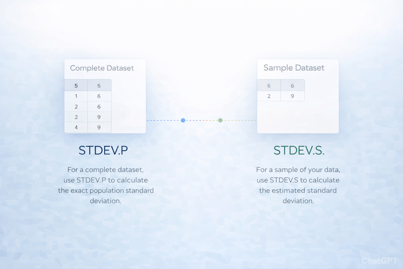
Method 1: STDEV.P in Google Sheets for a full population

1. Open your dataset in Google Sheets.
2. Confirm you truly have all records (e.g., every order from last quarter, not just a sample export).
3. In an empty cell, type: =STDEV.P(A2:A101) replacing A2:A101 with your range.
4. Press Enter. This is your population standard deviation.
5. Label the cell clearly: “Population stdev – full dataset” so teammates know why you chose STDEV.P.

Reference the Sheets function docs for details: https://support.google.com/docs/ (search “STDEV.P function”).

‍

Method 2: STDEV.S in Google Sheets for sample data

1. Open the sheet that holds a sample (e.g., 1,000 customers sampled from 50,000, or a subset of campaigns).
2. In an empty cell, type: =STDEV.S(A2:A1001)
3. Press Enter. This uses the n–1 method, giving a slightly larger, more honest estimate of variability.
4. Add a comment like: “Sample only – using STDEV.S for n–1 correction.”

‍

Method 3: STDEV.P in Excel

1. Open your workbook in Excel.
2. Confirm the data is the entire population you care about.
3. In a results cell, type: =STDEV.P(A2:A101)
4. Press Enter and format as needed.
5. For deeper reference, see Microsoft’s guide: https://support.microsoft.com/en-us/office/stdev-p-function-6e917c05-31a0-496f-ade7-4f4e7462f285

‍

Method 4: STDEV.S in Excel

1. For a sample-based sheet in Excel, select an output cell.
2. Type: =STDEV.S(A2:A1001)
3. Press Enter.
4. Note that this is the sample standard deviation (n–1). Documentation: https://support.microsoft.com/en-us/office/stdev-s-function-7d69cf97-0c1f-4acf-be27-f3e83904cc23

‍

Method 5: Z-scores in Sheets or Excel

Once you have a standard deviation, you can standardize any value x:

1. Compute the mean:
   • Sheets: =AVERAGE(A2:A101)
   • Excel: =AVERAGE(A2:A101)
2. Suppose mean is in B1 and stdev in B2. For a value in A2, enter: =(A2-$B$1)/$B$2
3. Fill down the column to get Z-scores. These help compare leads, campaigns, or product prices relative to the pack.

Manual methods are precise but fragile: every new sheet, export, or teammate can reintroduce formula mistakes.

‍

2. No-code methods with automation tools

Once your formulas are correct, you can reduce repetitive work – imports, updates, report refreshes – using no-code tools.

‍

Method 6: Live standard deviation dashboards in Google Sheets

1. Centralize raw data: use Google Forms, CSV imports, or CRM connectors (e.g., HubSpot → Sheets via native integrations or tools like Zapier/Make).
2. On a “Metrics” tab, set up:
   • =STDEV.S(...) for survey samples or test groups.
   • =STDEV.P(...) for “all orders last month” style datasets.
3. Use Named ranges (Data → Named ranges) like Orders_Amount and Survey_Scores to make formulas readable.
4. Add charts that reference these cells so standard deviation updates in real-time as data flows in.

‍

Method 7: Automate data collection with Zapier or Make

1. In Zapier, create a Zap: Trigger = “New row in Google Sheets” from an intake tab where raw data lands.
2. Action 1: “Create/update row” in a metrics tab where you keep a rolling list of values.
3. Because Sheets recalculates STDEV.P/STDEV.S automatically, your standard deviation metrics stay current without manual refreshes.
4. Optional: add an email/Slack step that posts a summary like: “This week’s NPS volatility (STDEV.S) is 1.3, up from 0.9.”

‍

Method 8: Template-driven rulebooks

1. Build a small “rule” table in Sheets:
   • Column A: Dataset name (Orders, Survey, Experiments, etc.).
   • Column B: Type (Population or Sample).
   • Column C: Formula tag (STDEV.P or STDEV.S).
2. Use simple IF logic in a metrics cell: =IF(VLOOKUP("Survey",Rules!A:C,2,FALSE)="Sample",STDEV.S(SurveyRange),STDEV.P(SurveyRange))
3. Now anyone adding a new dataset only has to set “Sample” vs “Population” once; the right function follows automatically.

No-code setups cut down on manual recalculation, but they still rely on humans to define the rules correctly – and to keep sheets consistent across teams.

‍

3. Scaling with an AI agent (Simular) across Sheets and Excel

At some point, you’re not just fixing one sheet – you’re inheriting dozens of dashboards across Google Sheets and Excel from sales, marketing, and ops. That’s where an AI computer agent like Simular becomes a force multiplier.

‍

Method 9: Audit and correct formulas at scale

How it works:

1. You give the Simular agent access to your Google Drive and key Excel workbooks.
2. The agent opens each file like a human: scanning cells, inspecting formulas, and reading labels.
3. It identifies where STDEV.P or STDEV.S is used, then cross-checks:
   • Tab name (e.g., “Full Orders 2024” vs “Orders Sample”).
   • Comments or documentation.
   • Row counts and filters (does it look like a subset?).
4. For obvious mismatches (“Survey Sample” using STDEV.P), it proposes or directly applies corrections and leaves a note.

Pros:

• Removes hidden formula landmines across dozens of sheets.
• Transparent execution: you can read every action the agent took.

Cons:

• Requires initial onboarding: which workbooks matter, and how conservative the agent should be about edits.

‍

Method 10: End-to-end reporting workflows

Scenario: A marketing agency runs weekly A/B tests for multiple clients.

Agent workflow:

1. Every Monday, Simular opens each client’s Sheets and Excel files.
2. It imports fresh data from analytics tools or CSV uploads, normalizes ranges, and recalculates:
   • STDEV.S for experiment groups.
   • STDEV.P where the client tracks a full user base.
3. It computes Z-scores for key KPIs (CPC, ROAS, conversion rate) and highlights outliers.
4. It drafts a short summary in a Google Doc or email: “Variation in Campaign B’s CPA (STDEV.S = 3.4) is double last week; recommend pausing low-performing ad sets.”

Pros:

• Frees sales/marketing from spreadsheet babysitting.
• Production-grade reliability: the same hundreds or thousands of steps run consistently.

Cons:

• You must define guardrails: which accounts, date ranges, and thresholds the agent uses.

‍

Method 11: Continuous quality monitoring

For finance, ops, or product teams, Simular can:

1. Nightly, open Sheets/Excel quality logs.
2. Recompute STDEV.P for full production metrics and STDEV.S for sampled QA checks.
3. Compare volatility week-over-week and flag anomalies in Slack.

This is the leap from “we have formulas” to “we have a tireless analyst” who never forgets when to use STDEV.P vs STDEV.S and documents every click.