How to Use Google Sheets VAR for Revenue Insights

1. Manual ways to calculate variance in Google Sheets

Before you automate anything, you need to be fluent in the basics. Google Sheets gives you several built‑in variance functions. The core reference from Google is here: https://support.google.com/docs/answer/3094063

‍

1.1 Using VAR (or VAR.S) on a sample

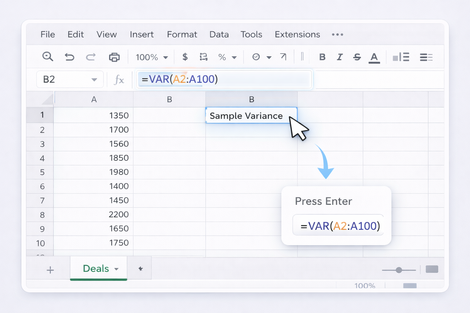
If you have a sample of data (e.g., last month’s deals), use VAR or VAR.S:

1. Put your numeric data in a single column, say A2:A100.
2. Click an empty cell where you want the variance, e.g., B2.
3. Type:
4. =VAR(A2:A100)
5. or the newer equivalent:
6. =VAR.S(A2:A100)
7. Press Enter. Sheets computes the sample variance by taking the squared deviations from the mean, divided by n-1.

Use this when you’re analyzing a subset of a larger population—like leads from just one campaign.

‍

1.2 Using VARP (or VAR.P) for full population

When your data represents the entire population (e.g., all invoices this year), use VARP or VAR.P:

1. Select an output cell, e.g., B2.
2. Enter:
3. =VARP(A2:A100)
4. or:
5. =VAR.P(A2:A100)
6. Press Enter. This divides by n instead of n-1, slightly reducing the variance.

‍

1.3 Manual variance calculation for learning

To really understand what’s happening under the hood:

1. In B2, calculate the mean:
2. =AVERAGE(A2:A100)
3. In C2, compute each deviation:
4. =A2 - $B$2
5. In D2, square that deviation:
6. =C2^2
7. Drag C2 and D2 down to row 100.
8. In a new cell, say E2, compute:
9. =SUM(D2:D100)/(COUNT(A2:A100)-1)

You’ve just replicated VAR.S manually. This transparency is powerful when you’re explaining the math to a non‑technical stakeholder.

‍

1.4 Variance across multiple ranges

VAR accepts multiple ranges:

=VAR(A2:A50, C2:C50, E2:E50)

Just remember Google’s note: VAR works across arguments as one combined sample; it does not return a separate variance per column.

‍

1.5 Pairing variance with STDEV and charts

1. Use =STDEV(A2:A100) (or STDEV.S) to get the standard deviation.
2. Insert a line chart (Insert → Chart) to visualize your series.
3. Use conditional formatting to highlight outliers more than 2 standard deviations from the mean.

This turns raw variance into a visual risk radar for your metrics.

‍

2. No‑code automation methods

Manual steps are fine for a single sheet. But business owners and agencies quickly drown in 20+ client tabs and weekly refreshes. No‑code tools can orchestrate the boring parts while you still stay inside Google Sheets.

‍

2.1 Use ARRAYFORMULA for auto‑filling variance

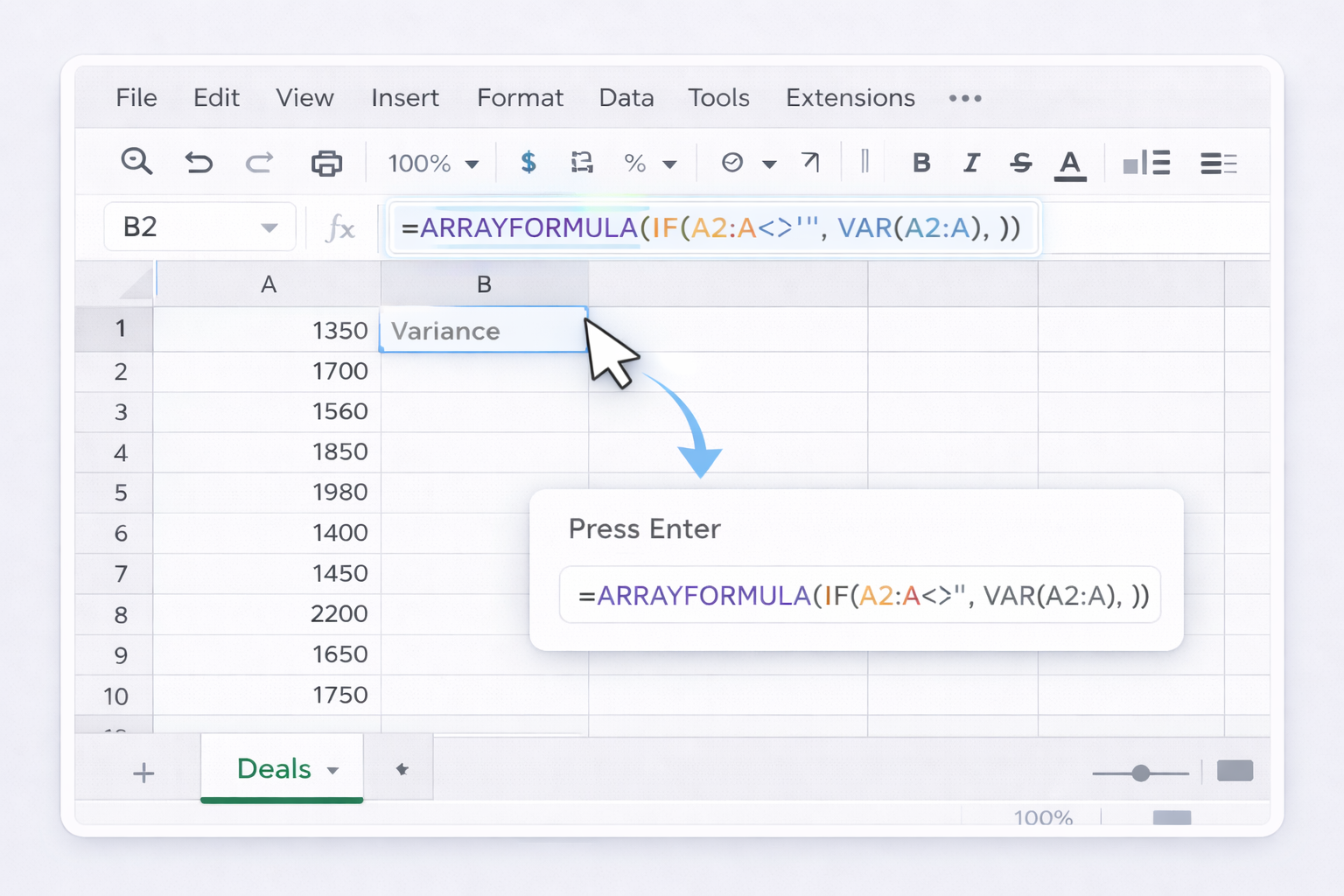
Instead of dragging formulas every week, let Sheets handle new rows automatically.

1. In B1, label it Variance.
2. In B2, enter:
3. =ARRAYFORMULA(IF(A2:A<>"", VAR(A2:A), ))

For many real‑world cases, you’ll structure data differently (e.g., one row per month). But the idea is consistent: ARRAYFORMULA applies your logic to entire ranges, recalculating as new data arrives.

Google’s guide to ARRAYFORMULA: https://support.google.com/docs/answer/3093275

‍

2.2 Scheduled refresh with connected data

If your data comes from BigQuery or other sources:

1. Use Data → Data connectors → Connect to BigQuery to pull data into Sheets.
2. Base your VAR() or VARP() formulas on the imported range.
3. Configure scheduled refresh (in the connector sidebar) so your variance updates automatically every day.

This is ideal for recurring KPI variance across marketing channels or sales regions.

‍

2.3 Combine variance with no‑code platforms

Tools like Zapier, Make, or Coefficient can:

• Pull CRM or ad platform data into Sheets on a schedule.
• Append new rows to a fact table.
• Trigger Slack or email alerts if variance crosses a threshold.

For example, a Zap could run daily, append yesterday’s ad spend and conversions into A2:B, and your existing =VAR.S(B2:B) instantly reflects the new volatility of CPA. No extra clicks from you.

‍

3. Scaling variance with AI agents (Simular)

Once you start tracking variance across dozens of metrics, tabs, and clients, even no‑code tools feel brittle. This is where an AI computer agent like Simular Pro takes over the actual computer work.

Learn more about Simular Pro: https://www.simular.ai/simular-pro About Simular’s approach: https://www.simular.ai/about

‍

3.1 Agent‑driven spreadsheet maintenance

Imagine your operations lead, but as software:

• The Simular agent opens Chrome, navigates to Google Sheets, and logs in.
• It locates a client’s performance workbook using the search bar.
• On each monthly tab, it inserts or updates formulas like =VAR.S(C2:C31) for revenue, =VAR.S(D2:D31) for CAC.
• It applies your preferred formatting (green for low variance, red for high).
• It writes a short text summary in a notes column: “CAC variance increased vs last month; paid social unstable.”

‍

Pros:

• Works across browser, desktop, and cloud tools exactly like a human.
• Fully transparent: every click and keystroke is logged and editable.
• Handles thousands of steps and many workbooks reliably.

‍

Cons:

• Requires an initial setup of a “golden” workflow for the agent to follow.
• Best value when you have repeatable, recurring reporting tasks.

‍

3.2 Multi‑client variance reporting at scale

For agencies or RevOps teams, Simular can:

1. Open a client index sheet with URLs to 50+ Google Sheets reports.
2. For each URL, open the sheet, duplicate a “Variance Report” template tab, and wire up VAR/VAR.P formulas to the right ranges.
3. Export summary tables to a central master sheet or CSV.
4. Trigger a webhook back into your production pipeline so the new report can be emailed, pushed to Slack, or surfaced in a dashboard.

‍

Pros:

• Massive time savings when you manage many similar workspaces.
• Fewer copy‑paste errors than manual or partially automated approaches.
• Easy to inspect and modify when business logic changes.

‍

Cons:

• You still need to define the logic for thresholds and alerts.
• Works best when your Google Sheets structure is reasonably standardized.

‍

3.3 Closed‑loop variance monitoring

With Simular Pro’s production‑grade reliability and webhooks, you can close the loop:

• Agent runs daily, recalculates variance on key metrics across Sheets.
• If variance for a KPI exceeds a limit, the agent logs into your CRM or ad platform to pull additional context (e.g., which campaign spiked).
• It posts a summary into Slack or email, with links to the exact Google Sheet tabs.

At this point, “calculating variance in Google Sheets” is no longer a task on your to‑do list. It’s an autonomous workflow that your AI computer agent owns end‑to‑end, while you focus on what matters: deciding what to do about the variance it finds.