
Oops! Something went wrong while submitting the form.
.svg)
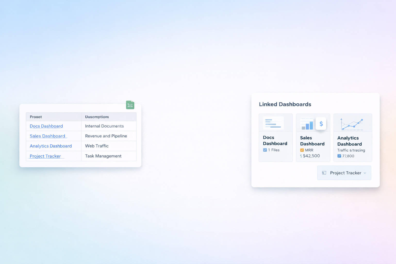
In every growing business there’s a moment when your Google Sheets go from neat tables to a maze of scattered URLs: CRM records, landing pages, proposals, tracking links. Hyperlinks are the connective tissue that turns those raw grids into living dashboards. With functions like HYPERLINK(url, label) and inline links, Sheets lets you jump from a row straight into a doc, site, or email draft, keeping sales, marketing, and ops in the same flow.
But when you’re maintaining hundreds or thousands of links, clicking into each cell to paste and test URLs quietly becomes someone’s part-time job. This is where delegating to an AI computer agent changes the story. Instead of humans hunting for the right URL, the agent can read your brief, pull URLs from CRMs or docs, write HYPERLINK formulas, apply link formatting, and verify each destination automatically. Your team stays focused on strategy, while the agent does the quiet, relentless work of wiring every cell to the right place, at scale.
If your team lives in Google Sheets—tracking leads, campaigns, or client projects—hyperlinks are how you turn a plain grid into a control panel. Let’s walk through three levels: manual basics, no‑code automation, and finally handing the whole thing to an AI agent so you never touch another tracking URL again.
These are the tactics your team probably already uses. They’re perfect for small sheets or one-off updates.
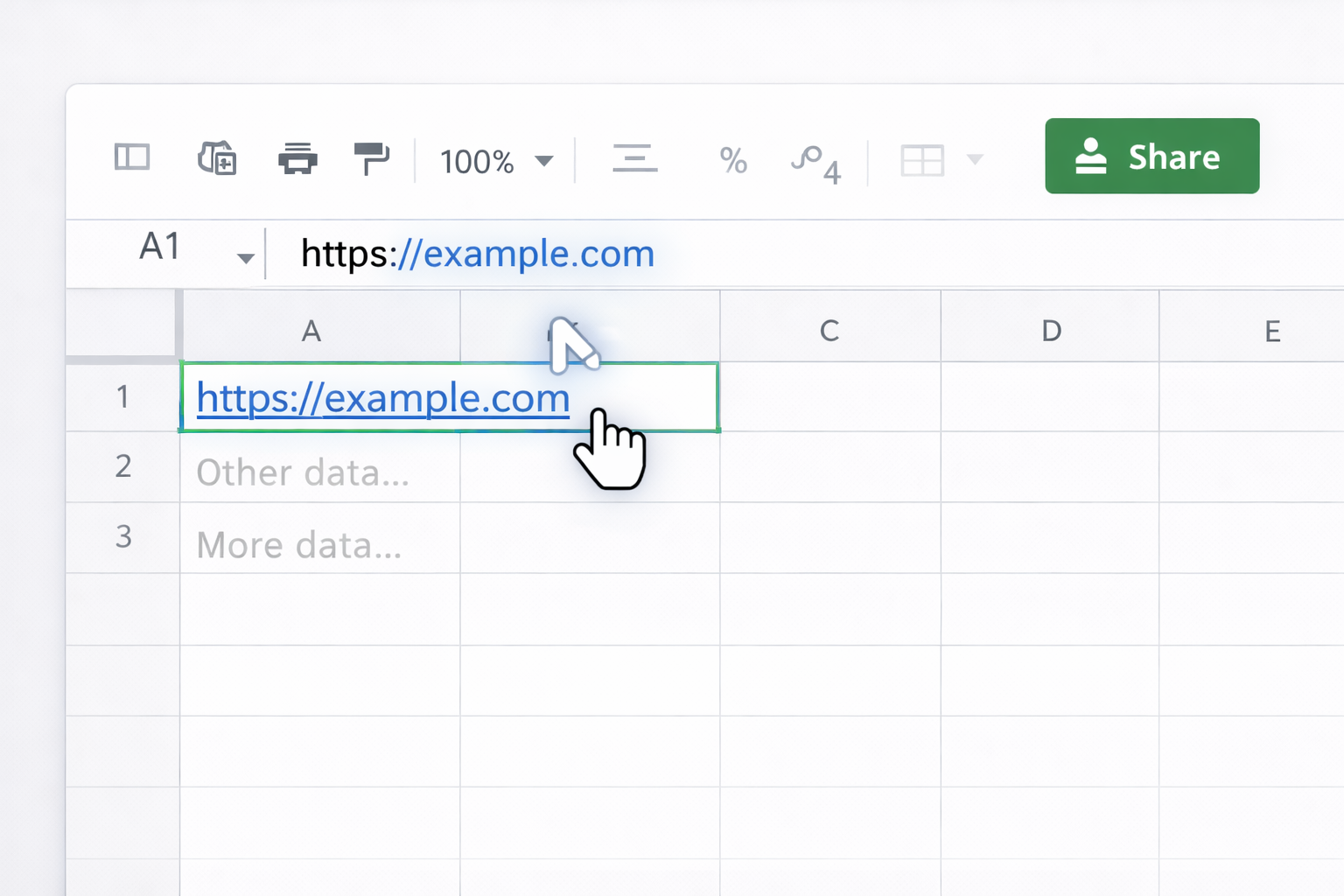
https://example.com.Pros: Fast, zero learning curve.
Cons: Ugly cell display, no friendly label text, unreliable if protocol is missing.
Official notes about supported link types are in Google’s HYPERLINK docs: https://support.google.com/docs/answer/3093313
This is the core formula for clean, labeled links.
Syntax (from Google Help):HYPERLINK(url, [link_label])
url: full URL in quotes or a cell reference.link_label (optional): readable text for the link.Example:
=HYPERLINK("https://www.google.com/","Google")
Step-by-step:
=HYPERLINK(."https://yourdomain.com".,"View page".) and press Enter.Docs: https://support.google.com/docs/answer/3093313
Pros: Clean labels, formula-driven, can reference other cells for dynamic URLs.
Cons: Editing long formulas gets messy, non-technical teammates may break them.
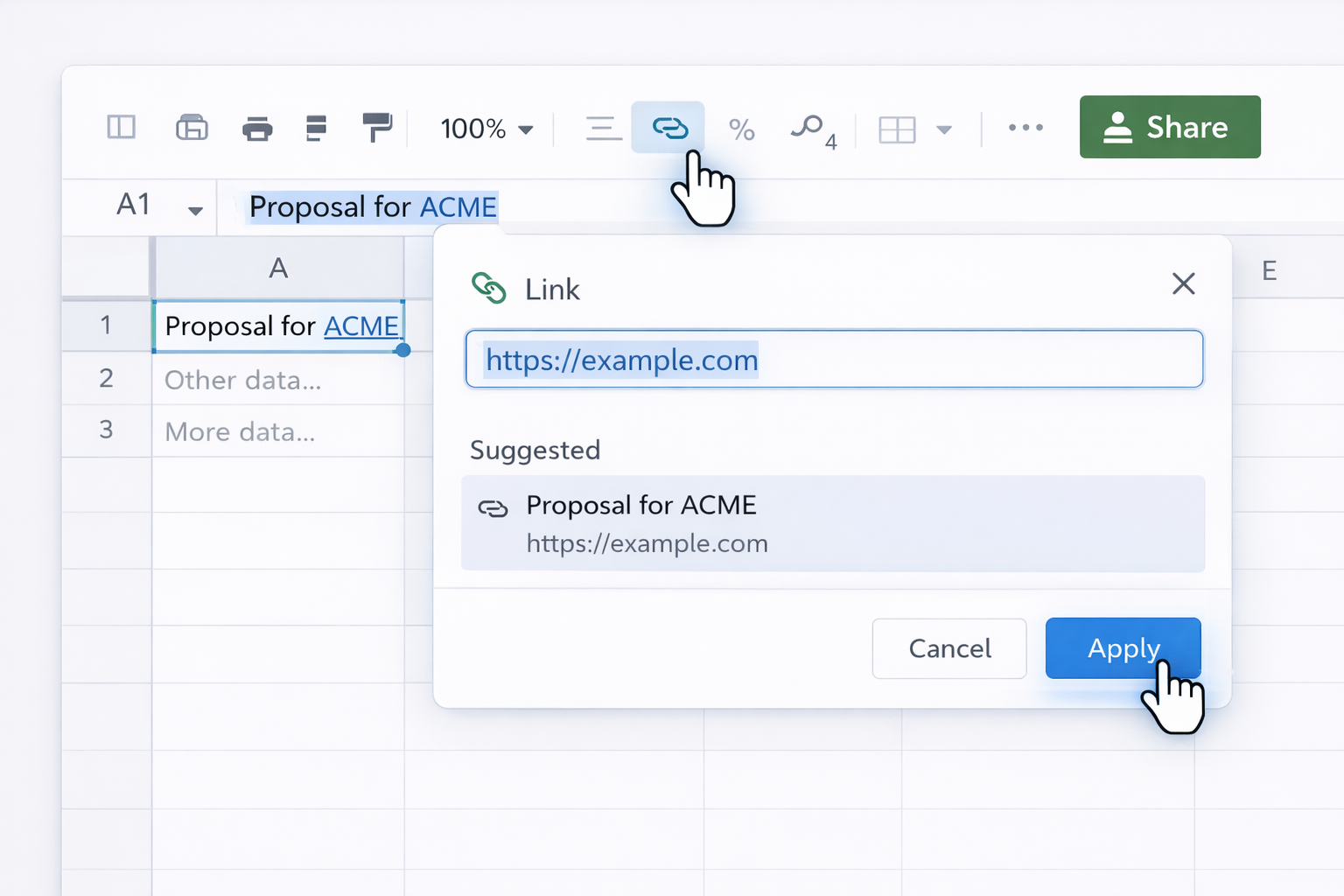
Use this for inline links or when you don’t want formulas cluttering cells.
Proposal for ACME.Google documents this behavior here (multiple links, inline text):
https://support.google.com/docs/answer/45893
Pros: Great for human-readable sheets, supports multiple links in a single cell.
Cons: Less transparent than formulas, harder to bulk edit or audit.
Sometimes the “URL” is another tab or range.
This is powerful for internal navigation dashboards—click a client name, jump to their detail tab.
You can join text and HYPERLINK in the same cell using concatenation functions.
Example:
="Deal: " & HYPERLINK(A2, "open CRM record")
Note: the hyperlink itself still applies to the full HYPERLINK result; you can’t make only one word clickable via formula. For granular inline links, you must select the text and use Insert → Link.
Reference discussion:
https://stackoverflow.com/questions/8970391/how-can-i-create-a-hyperlink-in-the-middle-of-cell-text
Once you’re managing dozens or hundreds of rows—like outreach lists, UTM links, or asset libraries—manual linking breaks down. Here’s how to level up without writing code.
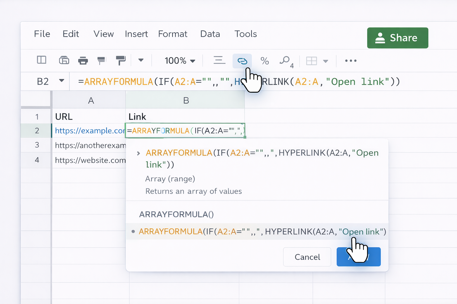
If you have URLs in one column and want labeled links in another:
A2:A).B2, enter:=ARRAYFORMULA(IF(A2:A="","",HYPERLINK(A2:A,"Open link")))
Pros: One formula powers an entire column.
Cons: Requires careful structure; teammates can accidentally overwrite array ranges.
For repetitive patterns (e.g. linking by ID), use a hidden “template” column.
Settings!B1 = "https://crm.yourapp.com/deals/".=HYPERLINK(Settings!B1 & A2, "Open deal")
A2:A are always present and valid.This avoids pasting full URLs and gives you central control of link structure.
If you’re feeding links into email tools or add-ons (like Yet Another Mail Merge), you can store personalized URLs per contact.
Google’s example shows using =HYPERLINK() or the toolbar to create HTML anchors that tools convert into clickable links in outgoing emails:
https://support.google.com/docs/answer/44660
CONCAT or & to assemble full URLs.HYPERLINK() where needed for humans; keep raw URLs for your mail-merge tool.
You can use tools like Zapier or Make to auto-fill hyperlink formulas when new rows appear.
Typical flow:
=HYPERLINK() formula.
Pros: Great for small automations, no engineering required.
Cons: Each run costs tasks/operations; debugging at scale can be painful; logic lives outside the sheet.
Official Google Sheets API docs (for tools that integrate via API):
https://developers.google.com/sheets/api
At some point, you’re not just “adding a few links”—you’re:
This is where an AI computer agent, like Simular Pro, becomes a real teammate.
Simular Pro is designed to behave like a power user across your whole computer environment—desktop, browser, and cloud apps. For hyperlink work, you can:
HYPERLINK() formula or insert an inline link.
Pros:
Cons:
Learn more about Simular Pro’s desktop and browser automation:
https://www.simular.ai/simular-pro
Hyperlink chaos kills trust in your Sheets. An AI agent can:
HYPERLINK() formulas using consistent labels (e.g. “Open deal”, “View doc”).
Here’s a practical play:
https://app.yourcrm.com/deals/”.
Because Simular Pro supports webhooks and integrates into existing pipelines, you can have:
For high-volume operations (agencies, sales orgs, RevOps teams), this shifts hyperlink management from “someone’s tedious side job” to an invisible, reliable background process—run by an AI computer agent that works at machine speed but behaves like a careful analyst.
