
Oops! Something went wrong while submitting the form.
.svg)
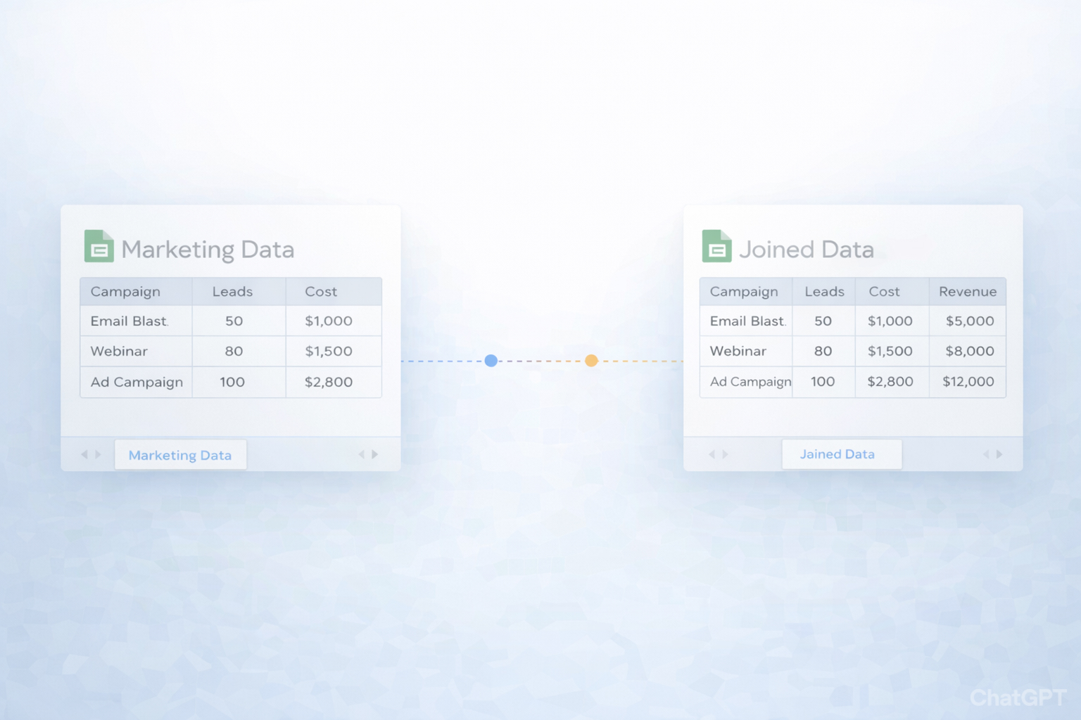
Every team has that one monster spreadsheet: leads from one form, campaign tags from another tool, and revenue data in a third tab. None of it lines up. The JOIN function in Google Sheets exists exactly for this moment. It lets you concatenate values from ranges using a consistent delimiter, so you can turn scattered cells into clean, readable strings for reporting, segment names, UTM lists, or CSV-style exports.
Used well, JOIN becomes the connective tissue of your sheets: combining first and last names, stitching together lookup keys, or collapsing long ranges into a single, human-friendly cell. But doing this repeatedly across dozens of tabs, files, and client accounts quickly turns into tedious, error-prone work.
This is where delegating to an AI computer agent matters. Instead of a marketer staying late to copy formulas and drag fill handles, an AI agent can open Google Sheets, apply JOIN and related functions, validate the outputs, and document what it changed. You get consistent joins, zero fatigue, and a workflow that can run every night while you focus on strategy and creative.
Think of manual methods as your "first gear". They’re perfect when you’re prototyping a report or handling a small list.
JOIN is built for turning many cells into a single, neatly formatted string.
Example: combine first and last name
A2:A, last names in B2:B.C2, enter: =JOIN(" ", A2, B2)Now each row contains a full name like Alex Chen.
Example: join a range into one comma-separated cell
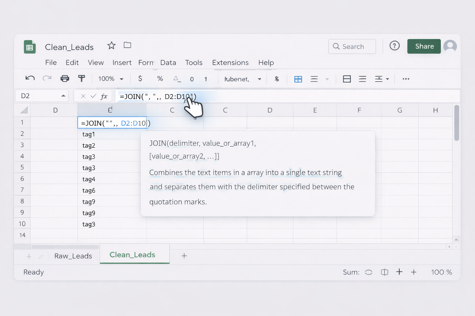
D2:D10.=JOIN(", ", D2:D10)tag1, tag2, tag3, ... in one cell.See the official docs for syntax details: https://support.google.com/docs/answer/3094077
& operatorIf you’re only joining a few cells, you can skip JOIN and use &:
C2, enter: =A2 & " " & B2Pros: very explicit and easy to debug. Cons: gets messy when you’re joining many cells or changing delimiters.
Sometimes you need to "join" data across two sheets, like matching CRM leads to billing data. You can’t do a true SQL join in native Sheets, but you can emulate it.
Step-by-step with helper keys:
Leads, create a key column K with: =A2 & "|" & B2 (e.g., email + country)Billing, create the same style key in column K.Leads!L2, use VLOOKUP against Billing: =VLOOKUP(K2, Billing!K:Z, 2, FALSE)JOIN isn’t doing the matching itself here, but it helps you build robust composite keys that power your lookups.
For very small datasets:
& columns to format final values.Pros: quick for < 50 rows. Cons: no audit trail, easy to misalign columns, impossible to scale.
IMPORTRANGE + VLOOKUPTo approximate a left join (all rows from Sheet A, matched data from Sheet B):
IMPORTRANGE.A2, pull the left table (optional) with IMPORTRANGE.G), enter: =ARRAYFORMULA(IF(A2:A="","", VLOOKUP(A2:A, IMPORTRANGE("<URL_of_right_sheet>", "Sheet1!A:Z"), 2, FALSE)))This is more advanced but still fully manual and formula-driven.
For more on combining ranges and functions, see the Sheets help center: https://support.google.com/docs
When you’re a founder or agency owner, you rarely have time to babysit formulas. No-code tools sit between "spreadsheet-only" and "full AI agent" and are ideal when your logic is stable but your data volume is growing.
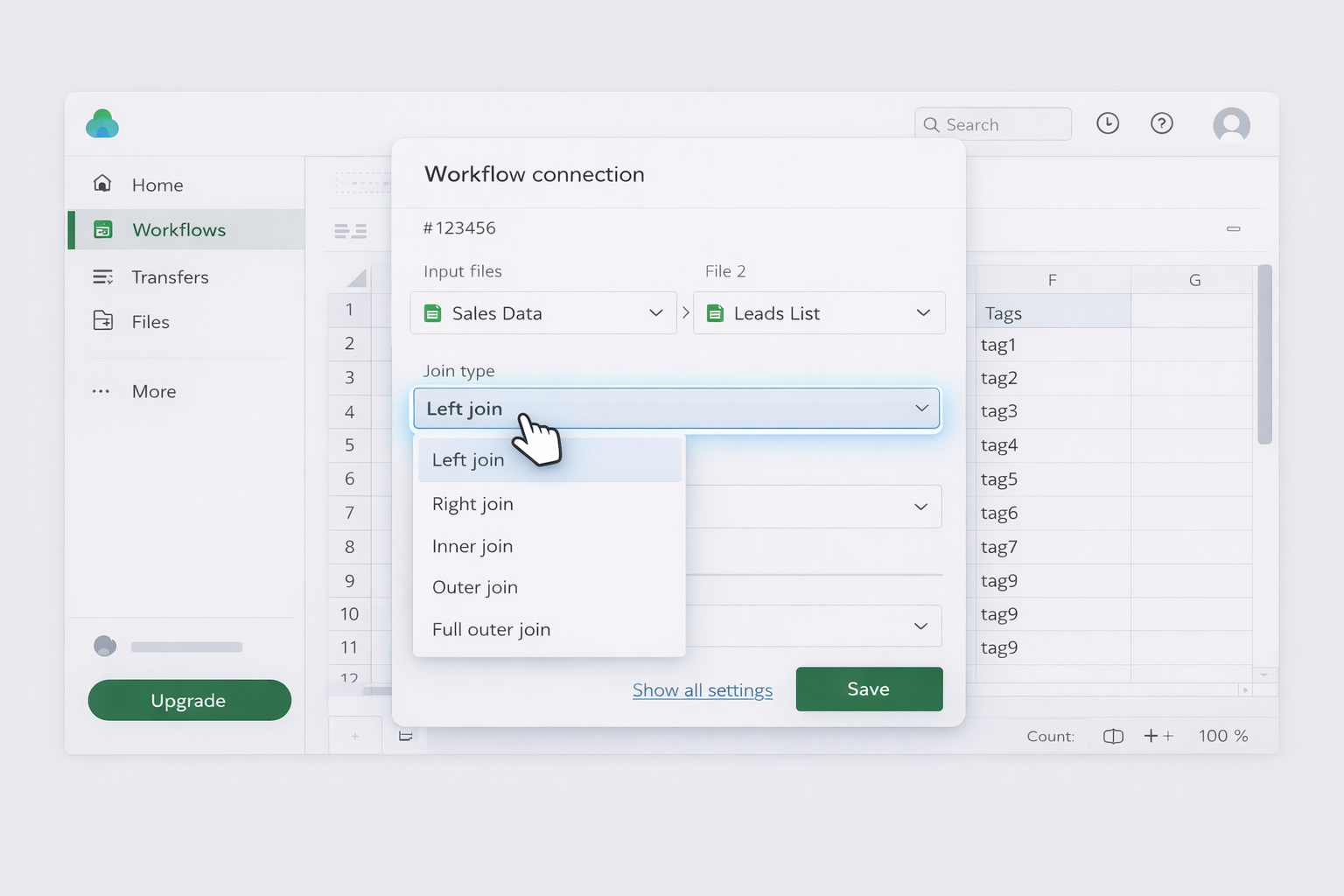
Sheetgo provides a visual way to combine multiple Google Sheets, including left joins.
Set it up:
Full guide: https://www.sheetgo.com/blog/how-to-solve-with-sheetgo/how-to-left-join-two-google-sheets/
Pros:
Cons:
Tools like Coefficient focus on pulling live data from CRMs, ad platforms, and warehouses into Google Sheets.
Typical workflow:
TEXTJOIN to combine labels, tags, or dynamic filter strings.Pros:
Cons:
Manual and no-code tools are great until your workflows become truly multi-step: pulling from email, CRM, web apps, then shaping everything in Google Sheets for each client. That’s where an AI computer agent, such as one powered by Simular Pro, becomes your operations teammate.
With a computer-use agent, you describe the workflow once; the agent then clicks, types, and navigates across your desktop and browser like a human.
Example workflow for an agency owner:
=A2 & "|" & B2).VLOOKUP/IMPORTRANGE-based pseudo joins.#N/A, blanks) and logs issues into a "Data QA" tab.Pros:
Cons:
Simular-style agents don’t stop at Sheets. They can:
SPLIT, CONCATENATE) to normalize fields (e.g., building a unified campaign_key from platform, country, and offer).Pros:
Cons:
Imagine telling your AI agent: "Every night at 1 a.m., clean all our client reporting sheets." The agent can:
Over time, this becomes an invisible ops layer that keeps your Google Sheets universe joined, consistent, and ready for analysis—without a human ever dragging a fill handle again.

